NeoStormer

Statistical Testing of the Hamamatsu UVTRON

MENG 572 - SENSOR TECHNOLOGY
STATISTICAL ANALYSIS OF A STATIC MEASURAND
TECHNICAL REPORT
SEPTEMBER 27, 2011


ABSTRACT

The object of this experiment is to determine how many readings of the Hamamatsu UVTron sensor are required to make a reliable decision of whether or not a flame is present. The experimentation consists of a LEGO Mindstorms NXT brick, a Hamamatsu UVTron, an adapter circuit, and custom specialized software NXTuary. An experiment was performed to determine the best number of readings necessary to make a decision; successful readings were counted out of ten readings for each test, and one hundred tests were performed. Statistical Characteristics were found for a group of thirty tests, and Statistical Classes were determined using Sturgis Rule. Statistical data was then graphed and a histogram was made to compare results to the Gaussian distribution. A 99% confidence interval was calculated to determine the minimum and maximum readings to be made during tests. The results showed that 4-6 readings per test would be sufficient to call the sensor detection accurate.


1. INTRODUCTION

This particular project was chosen because previous testing of using a Hamamatsu UVTron to find a flame proved quite unreliable. This experiment will determine how many readings of the sensor are required to make a reliable decision. The flame is not always detected during a single reading but can be using multiple readings, however more reading requires less more time. During a time trial of a robot, the less time required in detecting a flame means a faster accomplishment of the task. By knowing the statistical distribution of the measurand, a reliable reading can be made in less time. The UVTron measures Ultraviolet (UV) light and outputs a voltage, the output is either High or Low; therefore each reading is true or false.


2. THEORETICAL BACKGROUND

For this experiment: 100 Tests will be made, each test will take 10 readings and 30 of the tests will be chosen to be statistically analyzed. Statistical Characteristics will be found and Statistical Classes will be determined using Sturgis Rule. Once this step is completed, statistical data will be graphed and a histogram will be made to compare results to the Gaussian Distribution. A 99% confidence interval will be calculated to determine the minimum and maximum readings to be made during tests, thus solving the prior issues with the UVTron.


3. EXPERIMENTAL TESTING

3.1 INSTRUMENTATION

The following instruments were used in the experiment:

LEGO Mindstorms NXT



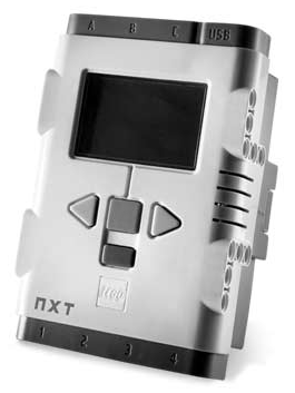
Figure 1: NXT Intelligent Brick
(Photo courtesy of LEGO)

The LEGO Mindstorms NXT is a programmable robotics kit released by LEGO in late July 2006. It replaces the first-generation LEGO Mindstorms kit, which was called the Robotics Invention System. This particular version is the Retail Version #8527. The main component in the kit is a brick-shaped computer called the NXT Intelligent Brick. It can take input from up to four sensors and control up to three motors, via RJ12 cables, very similar to but incompatible with RJ11 phone cords. The brick has a 100x64 pixel monochrome LCD display and four buttons that can be used to navigate a user interface using hierarchical menus. It also has a speaker and can play sound files at sampling rates up to 8 kHz. Power is supplied by 6 AA (1.5 V each) batteries or by a Li-Ion rechargeable battery.


UVTron Sensor



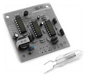
Figure 2: UVTron Driving Circuit and Sensor Bulb
(Photo courtesy of Hamamatsu Photonics)

The Hamamatsu flame sensor UVTron R2868 sensor package features a UVTron bulb. The detector makes use of the photoelectric effect and the gas multiplication effect. This works by UV light hitting a filament in a bulb attached to the board; as this occurs electrons are discharged into a thin plate, which is then converted by the on board electronics to a useable voltage. It has a spectral sensitivity of 185 to 260nm. The UVTron bulb is attached to the UVTron Driving Circuit C3704. The circuit allows the flame sensor to operate a low input voltage between 6 to 30V value.


Adapter Board



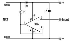
Figure 3: Adapter Circuit

Since the NXT uses a two data-power wire system (using the black and white wires) and the UVTron uses a three-wire system (power, ground and data), an adapter had to be created to separate the data wire from the power wires. This is done by the use of a 1kΩ resistor, a 1N4148 diode, an operational amplifier, a 22uF 16V capacitor, and a LM324 Quad op-amp. The schematic can be seen in Figure 3.


Software



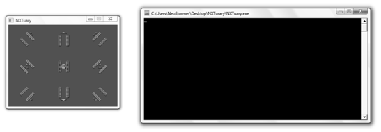
Figure 4: User Interface for the Control Screen in the NXT Software

Any software capable of interacting with the NXT would suffice, however particular software was chosen for this experiment due to its ease of use. The Bluetooth Remote Programming Software "NXTurary" (Previously known as "InterNXT") is a custom designed software that allows the NXT to be used as a remote data-logging device. While most NXT software use the onboard processing and storage memory to store and run programs, this software allows the computer to be used for processing and storage and remotely control the NXT (using Bluetooth) either through user input or programming lines; as the computer runs through the program it informs the NXT of what it needs to do such as read sensors or run actuators. By using this type of software, the limitations of the NXT are removed and therefore, it is only bound by the limitations of the user's computer. This software is developed by myself (Paul NeoStormer) and is written in C++ using the Dev-C++ compiler by Bloodshed Software.


3.2 EXPERIMENTAL PROCEDURE



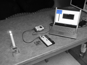
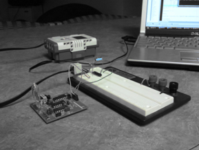
Figure 5: Setup of Experiment


Once the circuit is constructed and everything assembled; the NXT can be turned on.

The candle is then lit, placed approximately 1ft away from the UVTron detector, and the following program is run.

int test=100;

while(test>0)

{

    int count = 0, seen = 0;

    while(count<10)

    {

        count+=1;

        if (sensor1->read()<50)

        {

            seen+=1;

        }

    }

    cout << "#" << test << " I saw the flame " << seen << " times out of " << count << " tests" << endl;

    test-=1;

}

100 tests were performed (each test takes 10 readings), a sequential sample of 30 tests was chosen.

3.3 EXPERIMENTAL DATA

Table 1: Experimental Data

Sample #	Statistical Data	Comments
1	5
2	6
3	4
4	3
5	7
6	2
7	1
8	8
9	9
10	1
11	3
12	5
13	7
14	9
15	2
16	4
17	5
18	7
19	6
20	3
21	5
22	4
23	5
24	6
25	5
26	5
27	5
28	4
29	6
30	2

4. DATA ANALYSIS AND INTERPRETATION

4.1 RANKED DATA

Table 2: Ranked Data

Ranked Data	Sample #	z=(x-mean)/STD
1	7	-1.789281714
1	10	-1.789281714
2	6	-1.318418105
2	15	-1.318418105
2	30	-1.318418105
3	4	-0.847554496
3	11	-0.847554496
3	20	-0.847554496
4	3	-0.376690887
4	16	-0.376690887
4	22	-0.376690887
4	28	-0.376690887
5	1	0.094172722
5	12	0.094172722
5	17	0.094172722
5	21	0.094172722
5	23	0.094172722
5	25	0.094172722
5	26	0.094172722
5	27	0.094172722
6	2	0.565036331
6	19	0.565036331
6	24	0.565036331
6	29	0.565036331
7	5	1.03589994
7	13	1.03589994
7	18	1.03589994
8	8	1.506763549
9	9	1.977627158
9	14	1.977627158

4.2 STATISTICAL CHARACTERISTICS

Table 3: Statistical Characteristics of the Sample Data Set

Character	Value
Mean	4.8
Median	5
Min	1
Max	9
STD	2.123757

4.3 STATISTICAL CLASSES

The number and size of classes were determined using Sturgis Rule:

N = 1+3.3*log(n) = 1+3.3*log(30) = 5.8745

∆_N=(Max-Min)/N= (9-1)/5.8745=1.3618

Since the only possible data range is 0-10 and can only contains whole integers, ΔN has been made equal to 1 and to allow for two values on either side, N is now equal to 10. So the Sturgis rule is somewhat appropriate for this experiment.

 
Table 4: Statistical Classes and Measurand Statistical Distribution

Statistical Class	Statistical frequency	Sample relative frequency	Cumulative frequency	z=(x-mean)/STD	Normal distribution	Normal cumulative distribution
0	0	0.0000	0.0000	-2.2601	0.0146	0.0146
1	2	0.0667	0.0667	-1.7893	0.0379	0.0368
2	3	0.1000	0.1667	-1.3184	0.0788	0.0937
3	3	0.1000	0.2667	-0.8476	0.1312	0.1983
4	4	0.1333	0.4000	-0.3767	0.1750	0.3532
5	8	0.2667	0.6667	0.0942	0.1870	0.5375
6	4	0.1333	0.8000	0.5650	0.1601	0.7140
7	3	0.1000	0.9000	1.0359	0.1098	0.8499
8	1	0.0333	0.9333	1.5068	0.0604	0.9341
9	2	0.0667	1.000	1.9776	0.0266	0.9760
10	0	0.0000	1.000	2.4485	0.0094	0.9928

4.4 GRAPHICAL VISUALIZATION OF STATISTICS DATA



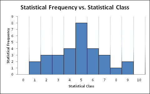
Figure 6: Statistical Frequency versus Statistical Class



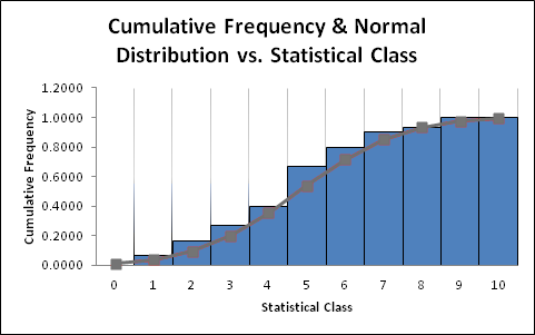
Figure 7: Cumulative Statistical Frequency and Normal Cumulative Distribution versus Statistical Class


4.5 COMPARISON TO THE GAUSSIAN DISTRIBUTION

While the plot is a Gaussian distribution, the variance appears to be off by quite a lot (this may be due to user error).



Figure 8: Experimentally Determined Statistical Frequency and Theoretically Calculated Normal Distribution for Statistical Classes of the Recorded Data

The data is almost exactly the same as the linear and the goodness of fit appears to be surprisingly close.



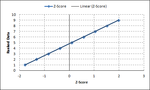
Figure 9: Statistical data versus the Z-score


4.6 EVALUATION OF CONFIDENCE INTERVALS

A 99% confidence interval shows that:

x ̅- t_(∝/2,n-1) s/√n ≤ μ ≤ x ̅+ t_(∝/2,n-1) s/√n

(4.8)-(3.04) ((2.123757))/√30 ≤ μ ≤ (4.8)+(3.04)((2.123757))/√30

3.621261 ≤ μ ≤ 5.978739

4 ≤ μ ≤ 6


5. DISCUSSION

These results have show that 4-6 readings would be sufficient enough to call the sensor detection accurate; this will result in time saved during trials. Potential errors include outside UV sources, even though this experiment was done inside during nighttime hours there could be a few outside sources. Distance to the flame could cause bias errors, the sensor can see up to 5 meters but during this experiment it was placed approximately 1ft away.


6. CONCLUSION

It has been determined that 4-6 readings per test will be sufficient to call the sensor detection accurate. The Measurand distribution is definitely Gaussian, it appears that an outlier appears to be at 9 true data readings during one test. The determined statistics appear to adequately represent the issue with the UVTron.


7. ACKNOWLEDGMENTS

Would like to thank RoboRAVE International (TM) for donating the sensor and their continuous support with these projects.


8. REFERENCES

Wilson, J.S. (editor), (2004) "Sensor Technology Handbook," Newnes, 1st edition.